Generate an entirely black image.
Use the following Python program, black_image.py, to create a 64x64 PPM image that is entirely black. Running the Python program will generate a 2-D array of RGB color values for the image. Each row of text in the output representes one row of pixels, and each set of 3 values represents the R, G, and B values for each of the 64 column pixels in that row (i.e. there are 3 * 64 values per row).
There are two ways you can run the program. The first option is to run it in a Linux console/terminal window by typing python black_image.py > black.ppm (in the directory containing the black_image.py program). This method uses the '>' operator to automatically redirect the output to the black.ppm image (so no additional work is needed to copy the output into an image file).
As an alternative, you can copy the program into the Python simulation environment and execute the program from there. Once you have generated the output, copy the header and the 64 rows of values (i.e. copy all the output except the ------ simulation is beginning ------ and ------ simulation is complete ------ lines of the output) into a text editor and save the file as black.ppm. The resulting file should be equivalent to black.ppm.
Open the black.ppm file with XnView, and it should display a small (64x64 pixel) black image. Use the Zoom In function of XnView, and zoom in a few times to get a better look at the image.
Generate a black image with a diagonal line of purple pixels.
In the inner loop in the Python program from above, change the line in black_image.py:
print "0 0 0",
to:
    if (x == y):
        print "255 0 255",
    else:
        print "0 0 0",
The resulting program should be equivalent to purple_diagonal_image.py.
Again, there are two ways you can run the program. The first option is to run it in a Linux console/terminal window by typing python purple_diagonal_image.py > purple_diagonal.ppm (in the directory containing the purple_diagonal_image.py program). This method uses the '>' operator to automatically redirect the output to the purple_diagonal.ppm image (so no additional work is needed to copy the output into an image file).
As an alternative, you can copy the program into the Python simulation environment and execute the program from there. Once again, copy the header and the 64 rows of values (i.e. copy all the output except the ------ simulation is beginning ------ and ------ simulation is complete ------ lines of the output) into a text editor and save the file as purple_diagonal.ppm. Upon viewing the image in XnView, you should see an image that looks like:

Generate a shaded image that progresses from black in the top row to bright blue in the bottom row of pixels.
In the inner loop in the Python program from above, change the line in black_image.py:
print "0 0 0",
to:
print "0 0", y * (256 / rows),
The resulting program should be equivalent to blue_shaded_image.py.
Again, there are two ways you can run the program. The first option is to run it in a Linux console/terminal window by typing python blue_shaded_image.py > blue_shaded.ppm (in the directory containing the blue_shaded_image.py program). This method uses the '>' operator to automatically redirect the output to the blue_shaded.ppm image (so no additional work is needed to copy the output into an image file).
As an alternative, you can copy the program into the Python simulation environment and execute the program from there. Once again, copy the header and the 64 rows of values into a text editor and save the file as blue_shaded.ppm. Upon viewing the image in XnView, you should see an image that looks like:

Generate the outline of a green box on a blue background, with each side 10 pixels from the edge of the image.
In the inner loop in the Python program from above, change the line in black_image.py:
print "0 0 0",
to:
    if (((y == 10) or (y == 53)) and ((x >= 10) and (x= 53))):
        print "0 255 0",
    elif (((x == 10) or (x == 53)) and ((y >= 10) and (y <= 53))):
        print "0 255 0",
    else:
        print "0 0 255",
The resulting program should be equivalent to green_box_on_blue_image.py.
Again, there are two ways you can run the program. The first option is to run it in a Linux console/terminal window by typing python green_box_on_blue_image.py > green_box_on_blue.ppm (in the directory containing the green_box_on_blue_image.py program). This method uses the '>' operator to automatically redirect the output to the green_box_on_blue.ppm image (so no additional work is needed to copy the output into an image file).
As an alternative, you can copy the program into the Python simulation environment and execute the program from there. Once again, copy the header and 64 rows of output from Python into a text editor and save the file as green_box.ppm. Upon viewing the image in XnView, you should see an image that looks like:

Some additonal Python examples:
-
blue_reverse_shaded_image.py produces an image that looks like:

-
blue_tic_tac_toe_image.py produces an image that looks like:

-
red_line_image.py produces an image that looks like:

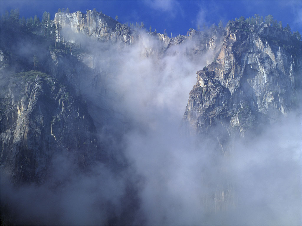
Compress an image using JPEG compression.
Download the image, Cliff_in_Clouds.bmp.
View the image in the XnView image viewing tool. Within XnView, under the File sub-menu, select Save As... This will open the Save picture window. At the bottom of this window, for the image type in Save as type:, select JPG - JPEG / JFIF. Then, before saving the file, select the Options button in the lower left-hand corner of the window. This opens the Options window. On the right side of the Options window, there's a sliding bar to select the Quality. Slide the bar to the left, until the Quality (in the small window to the right of the sliding bar) indicates 20. Then hit OK at the bottom of the window. This will close the Options window, saving the Quality level as 20 (out of 100). Finally, select Save in the Save picture window to save the image. This will create an image, Cliff_in_Clouds.jpg.
To compute the degree of compression, divide the file size of the original uncompressed file, Cliff_in_Clouds.bmp, by the file size of the new compressed file, Cliff_in_Clouds.jpg. The original size is 2359350 bytes (about 2.25 MB) and the compressed file should be 28640 bytes (about 28.0 KB). Therefore the degree of compression can be calculated as:
    degree of compression = 2359350 / 28640
                          = 82.4
In other words, the compressed file (using JPEG compression) is 82.4 times smaller than the original uncompressed file.
Compress an image using JPEG-2000 compression.
Download the image, Cliff_in_Clouds.bmp.
View the image in the XnView image viewing tool. Within XnView, under the File sub-menu, select Save As... This will open the Save picture window. At the bottom of this window, for the image type in Save as type:, select JP2 - JPEG-2000 JP2 File Format. Then, before saving the file, select the Options button in the lower left-hand corner of the window. This opens the Options window. On the right side of the Options window, there's a sliding bar to select the Quality. First select the radio button next to Quality, to make sure compression is being based on the Quality level. Then slide the bar to the left, until the Quality (in the small window to the right of the sliding bar) indicates 20. Then hit OK at the bottom of the window. This will close the Options window, saving the Quality level as 20 (out of 100). Finally, select Save in the Save picture window to save the image. This will create an image, Cliff_in_Clouds.jp2.
To compute the degree of compression, divide the file size of the original uncompressed file, Cliff_in_Clouds.bmp, by the file size of the new compressed file, Cliff_in_Clouds.jp2. The original size is 2359350 bytes (about 2.25 MB) and the compressed file should be 26897 bytes (about 26.3 KB). Therefore the degree of compression can be calculated as:
    degree of compression = 2359350 / 26897
                          = 87.7
In other words, the compressed file (using JPEG-2000 compression) is 87.7 times smaller than the original uncompressed file.


