Lab 05

Contents:

• Overview
• Files You Need
• Your Tasks
• Turtle Graphics Primer
• Algorithm Overview
• Warmup Questions
• draw1 function
• draw2 function
• Submitting Your Assignment
• Grading Standards

Our textbook authors prepared a series of labs associated with Chapters 9,10 of the text (part1, part2, part3, part4), and while you are welcome to go through those labs on your own time, there is something dissatisfying about the drawing algorithm that they suggest. While they look nice on the examples they use, such as with

the problem is that with larger trees, their algorithm does not disallow portions of one branch of a tree from overlapping the visualization of another branch of the tree. For example, applying their algorithm to a more complex tree produces the following image:

While their algorithm, with sloped lines, could be remedied, we will instead explore a different visualization style that uses orthogonal lines, producing images such as the following for the above examples:

For full disclosure, this example is modeled from an example in a 2011 article Megacycles of atmospheric carbon dioxide concentration correlate with fossil plant genome size.

We are providing you with two files:

• treeViz.py
  We have provided some utility functions to get you started, and we have stubbed out the draw1 and draw2 functions which you are to implement.

• samples.py
  This file provides a variety of sample trees for use in testing your software (many of which are described below as examples).

There will be three requirements for your submission of this lab, each of which is described in far more detail in the remainder of this document.

• Warmup questions
  Before doing any coding, we need you to better understand the recursive nature of the drawing algorithm, so we will ask you to do some pen-and-paper examples (but to later type up your answers within comments of your source code).

• draw1 function implementation
  Then you will implement the first version of the drawing algorithm.

• draw2 function implementation
  We will guide you through a more advanced refinement of the algorithm that varies edge lengths to match presumed evolutionary time period.

The turtle module is part of Python's standard libraries, to provide an illustrative way to generate some basic graphics. The turtle is effectively a virtual robot with a pen that draws lines as it moves. The only behaviors you will need to use are:

• turtle.forward(distance)
• turtle.backward(distance)
• turtle.left(degrees)
• turtle.right(degrees)
• turtle.write(message)

For convenience in testing, we have provided a function reset() within our code that clears the screen and returns the turtle to a starting position near the left edge of the screen. You should call reset() just before starting your draw function (but not from within!).

Our drawings will be produced with a recursive algorithm. By convention, we will assure that when drawing a tree, the turtle begins facing rightward at the point that should become the left edge of the tree visualization, and with a vertical position that should be the vertical center of the eventual tree. Furthermore, we will assure that the leaves of the tree are to be laid out vertically at regular intervals (which we will denote as yScale within our later functions). For example, we might decide that leaves will be drawn at 20-pixel intervals on the vetical scale. By this convention, a generic schematic of a tree with eight leaves might appear as follows:

with the solid rectangle meant to portray the bounding-box of the tree, and the eight dashed horizontal lines designating the vertical location of where those eight leaves will eventually be drawn. Notice that the turtle starts precisely at the vertical center of the image.

With a recursive approach, the key insight is that if we have a tree that is a single leaf, we simply need to write the text information about the leaf. For any other tree, rather than worrying about all the complexity of the tree, we want to do the following basic steps:

1. Turn to move upward, then rightward, leaving the turtle at the appropriate starting spot for the first subtree.
2. Recursively draw that subtree (which must leave the turtle precisely located and oriented where it started).
3. Retrace the path to the root and then move downward, then rightward, leaving the turtle at the appropriate starting spot for the second subtree.
4. Recursively draw that subtree (which must leave the turtle precisely located and oriented where it started).
5. Retrace the path to the root and leave the turtle oriented facing rightward (just as we found it when beginning this process).

The key to the success of our algorithm (and avoiding overlap of subtrees) is in determining precisely how far upward/downward/rightward to move before restarting each recursive drawing. In determining how far upward/downward to move, we must rely on our convention that the eventual leaves of the tree be evenly spaced on the vertical scale. If we knew how many leaves were in the first and second subtree, we should be able to determine the correct vertical offsets.

As a first example, consider the generic 8-leaf tree and presume that we knew that the first subtree had 3 of those leaves and the second subtree had 5 of those leaves. In this case, we should envision the recursive process as follows:

Notice that the top of the two subtree bounding boxes will cover three of the eventual leaves and we will bring the turtle precisely to the center of the left edge of that bounding box before starting the recursion. The bottom of the two subtrees will have five leaves, and thus we can determine where the left-center of that box should be.

Of course, if we had a different distibution of leaves, we would need our algorithm to "deliver" the turtle to other locations. For example, here is a schematic for an 8-leaf tree with 6 leaves in the first subtree and 2 in the second.

For convenience, the Python code we are providing you with already has a function with signture leafCount(tree) that returns the number of leaves within a given tree or subtree.

This brings us to your first part of the lab. We must eventually come up with a programatic way to determine the various distances for a new tree that we encounter. But before getting bogged down in Python code, you need to work out some cases by hand, and then hopefully determine a pattern that will allow you to generalize this to arbitrary size trees.

The question at hand is if we assume that the turtle starts at coordinate y=0, we wish to determine what the y value should be for starting the first subtree and what the y value should be for starting the second subtree. For the sake of these examples, let's assume that the leaves are rendered 10 pixels apart from each other. (In our real code, we'll make that yScale a parameter.) Also, unlike mathemticians, computer scientists tend to count pixels from the top of the screen downward, and thus we consider moving upward in the negative direction and downward in the positive direction.

Revisiting our first example of an 8-leaf tree with 5 leaves in its first subtree and 3 in its other, the first subtree should begin at height y=-25 and the second at height y=+15. In the second example, with 6 leaves in the top and 2 in the bottom, the starting heights for the recursions were y=-10 and y=+30 respectively.

You must complete the following table (which we've placed within the comments of the source code we are providing).

total leaves	upper leaves	lower leaves	upper y-value	lower y-value
8	3	5	-25	+15
8	6	2	-10	+30
8	4	4
8	7	1
7	3	4
7	1	6
n	a	b

Note well that the last entry of this table is the most important, as you need to discover a formula that works for general parameters (presuming that a+b=n).

Now we are ready to write some code. We will do two versions of the visualization that differ in how they manage the horizontal spacing of the drawing. In the first version, we will simply move a fixed amount rightward for each level of the tree. The function should have signature

def draw1(tree, xScale, yScale):

The code for your implementation should follow the high-level algorithm enumerated above, distinguishing between a base case where you have a tree with empty subtrees and the general case in which the subtrees are nontrivial. The above turtle graphics primer can guide you through use of the graphics package.

We have included a variety of sample trees within the Python code. Here are some renderings for you to match:

Tree from Figure 9.3 of our book, rendered as draw1(fig93, 50, 50):

Tree from Figure 9.4 of our book, rendered as draw1(fig94, 50, 50):

Rendered as draw1(treeFrogs, 50, 50):

Rendered as draw1(complex, 40, 15):

The difference between the draw1 and draw2 functions involved the rightward spans of the edges when moving from a branch point to its subtrees. With draw1, we simply used a fixed increment for each rightward movement.

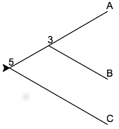
However, leaves of phylogetic trees are often based on relatively modern day samples of organisms, while internal nodes represent hypothesized common ancestors. Therefore, visualizations that one to capture the history align all of the leaves at the far right of the figure, and internal nodes can be augmented with a numeric value that estimates how long ago that common ancesstor branched. For example, in the following tree (named withLengths in the samples)

we might presume that the 3 denoted at the nearest ancestor to A and B suggests that existed 3 million years ago while the 5 denoting the common ancestor of that node and C occurred 5 million years ago. Internally, this tree is represented as follows.

(5,
   (3,
        ("A", (), ()),
        ("B", (), ())
   ),
   ("C", (), ())
 )

In the second version of our visualization, named draw2, we interpret the numbers at those internal nodes as ages, and modify the lengths of the horizontal edges to reflect the time scale, such that modern-day is thought of as time 0 at the far right and then other ancestors are separated based on the time gaps from the data. For example, the above tree would be rendered in our new format as

The length of the edges from A and B to their ancestor is equal to three units (times some arbitrary xScale factor that can be given as a parameter to convert to pixels), and the line from that ancestor back to the root is length two units (because that connects the ancestor that was modeled as 3 million years ago to the one that was 5 million years ago). More generally, when going from a parent to a child in the tree, the length of the edge should be proportional to the numeric "age" of the parent and the numeric "age" of the child (with leaves implicitly having age 0). The xScale parameter should not be a multiplier to the horizontal length.

Here are a few other examples that are included in our sample data sets. There is a data set about tree frogs from the textbook authors. Its internal numbers are shown on this rendering from draw2(treeFrogs, 50, 50):

Its new rendering as draw2(treeFrogs, 5, 50) appears as:

Finally, here was our rendering of the most complex tree in our data set, which we rendered with parameters draw2(complex, 1, 15):

One member of your partnership should electronically submit your modified file treeViz.py. The comments at the beginning of the file should clearly identify the member(s) of the partnernship and should include answers to the "warmup" questions.

The assignment is worth 10 points, which will be assessed as follows:

• (3 points) Correct answers to warmup questions.
• (5 points) Correct implementation of draw1 function.
• (2 points) Correct implementation of draw2 function.

Note well that the more advanced draw2 is worth a relatively small percentage, not because it is easy, but so that you are able to get 8/10 points just by correctly completing the warmup and the first implementation correctly.