CSCI-1080 Intro To CS: World Wide Web

Information, computation, and algorithms

Computer science is “the study of the theoretical foundations of information and computation” Wikipedia, 2016.

Examples of information include:

The Adventures of Huckleberry Finn, novel by Mark Twain
Results of the United States Census 2000
Letters of the alphabet

We will not attempt to define information. Instead, we simply note that sets and ordered lists, which we have already discussed, provide a basic foundation for the theory of information.

Computation is a form of action. Examples include:

Add the first 100 Natural numbers
Digitize a photograph as a JPG image
Sort a list of United States households according to their gross annual incomes
Find a shortest path (i.e., with fewest links) via the Internet from slu.edu to your browser

An algorithm is a step-by-step procedure for performing a computation. We introduced algorithms to illustrate network dynamics. Our repertoire of algorithms so far includes the random graph algorithm, the triadic closure algorithm, and the preferential attachment algorithm.

Summation: an example of what computation is

Adding a series of numbers, called summation, is a simple example of computation. Below is a basic algorithm for summation:

Summation Algorithm:

Input:

Integer n, with n > 0

Output:

Variable t =1+2+3+ … + n

Steps:

if then we are done
go to step 3

The symbol sum denotes summation and is used to represent calculations similar to the above.

Example: The simplest form of summation notation is

$sum_{i=1}^n i$

Given an integer n>0, the above notation represents the sum 1+2+3+…+n.

Example: We use sets to define a more general notion of summation. Let A = {1,2,3,…,n} with n>0. Then the previous example can also be written

$sum_{i in A} i$

Notice how the more general notation for summation is similar to implicit notation for sets. In the above example, the dummy variable is i and the true/false statement is i in A . The symbol sum denotes the summation of all values of the dummy variable for which the true or false statement is true.

Example: Let A = {1,5,8,20}. Consider

$sum_{{i in A} ;; and ;; {i ; is ;even}} i$

This is 8+20 = 28 .

Example: Let A = {2,4,8}. Consider

$r = sum_{{i in A} ;; or ;; {i =3}} i^2$

How much is ?

HTML: an example of what computation is not

HTML is arguably the fundamental computer language of the Web and the basis of Web programming; however, many computer scientists do not consider HTML to be a programming language.

The distinction between the popular notion of “Web programming” and the computer science notion of “programming language” hinges on computation. A computer scientist uses a programming language to express algorithms that do computation. In contrast, Web programming does not require the author to write algorithms to do computation.

For example, if you want to add the numbers 1+2+3+ldots+100 , then HTML is not helpful. Even the simplest arithmetic cannot be performed by HTML. The language is not designed to express algorithms of any kind.

HTML does not express algorithms, but it certainly does represent information. For example, if you wanted to write a story about adding the numbers 1+2+3+ldots+100 , then HTML provides a language with which you can tell that story. You could also use HTML to tell the story of The Adventures of Huckleberry Finn. Both of these stories are examples of information, not computation.

If you used HTML to write a story about adding the numbers 1+2+3+ldots+100 , then you would probably want to use an algorithm (expressed by some programming language other than HTML) in order to compute the actual sum. Then with HTML you could present that sum as a tidy conclusion to the story.

For example, you could use the Web scripting language PHP to add 1+2+3+ldots+100 and to generate the HTML that would present the above story. PHP can express algorithms that do computation; it is a programming language in the classic sense.

Examples of Algorithms seen so far

Random Graph Algorithm

Start with node set V with |V|>1
E = { }
 Choose random pair of nodes x, y that are non-adjacent
 Add element {x,y} to set E
If |E| = |V|*(|V|-1)/2 then we're done
Go to step 3

Random Graph Algorithm v2

Alternatively, we can stop when we have tried to add an edge for each couple of nodes:

Start with node set V with |V|>1
E = { }
counter = 0
     Choose random pair of nodes x, y that are non-adjacent
     counter = counter + 1
Add element {x,y} to set E
If counter = |V|*(|V|-1)/2 then we're done
Go to step 4

Triadic Closure Algorithm

Start with graph G=(V,E) with |V|>0 and |E|>0
Choose random pair of nodes x, y that are non-adjacent and share a common neighbor
If no such pair of nodes x, y exists, then we’re done
Add element {x,y} to set E
Go to step 2

Triadic Closure Bias Algorithm v1

1.	Start with:
	a.	T = bias toward triadic closure = number between 0 and 1 inclusive
	b.	graph G=(V,E) with |V|>0 and |E|>0
2.	"Flip a coin": r = random number between 0 and 1 inclusive
3.	If (r ≤ T)
		Choose random pair of nodes x, y that are non-adjacent and share a
		common neighbor
	Else
		Choose random pair of nodes x, y that are non-adjacent
4.	If no such pair of nodes x, y exists, then we’re done
5.	Add element {x,y} to set E
6.	Go to step 2

Triadic Closure Bias Algorithm v2

1.	Start with:
	a.	T = bias toward triadic closure = number between 0 and 1 inclusive
	b.	graph G=(V,E) with |V|>0 and |E|>0
2.	"Flip a coin": r = random number between 0 and 1 inclusive
3.	If (r ≤ T)
		Choose random pair of nodes x, y that are non-adjacent and share a
		common neighbor. The probability of choosing pair {x,y} corresponds
		to the number of neighbors that x and y share.
	Else
		Choose random pair of nodes x, y that are non-adjacent
4.	If no such pair of nodes x, y exists, then we're done
5.	Add element {x,y} to set E
6.	Go to step 2

Triadic Closure Bias Algorithm v3

1.	Start with:
	    a. T = bias toward triadic closure = number between 0 and 1 inclusive
	    b. graph G=(V,E) with |V|>0 and |E|>0
2.	"Flip a coin": r = random number between 0 and 1 inclusive
3.	If (r ≤ T)
              Choose random pair of nodes x, y that are non-adjacent and share a
              common neighbor. The probability of choosing pair {x,y} corresponds
              to |N(x) ∩ N(y)| / |N(x) U N(y)|.
	Else
              Choose random pair of nodes x, y that are non-adjacent
4.	If no such pair of nodes x, y exists, then we’re done
5.	Add element {x,y} to set E
6.	Go to step 2

Computing distance, part one

Given an undirected graph G=(V,E) , we previously defined the distance between two nodes x and y as the length of a shortest path in G from x to y. Now we describe how to compute this value.

Computing distance in a graph relates to several important topics in Web science:

Information diffusion: how does information spread over time through a population of Web users?
Packet routing: how is a discrete piece of information transmitted between two computers via the Internet?
Network navigation: how does one explore the connections in a network? (See “broadcast search” and “directed search” in Six Degrees for more on this).

Computing distance in a graph is also very closely related to computing shortest paths in a graph. Finding shortest paths is a fundamental problem in computer science that is traditionally solved with breadth-first search. Our distance algorithm is a slightly simplified version of breadth-first search.

We motivate our distance algorithm with the following scenario:

Suppose m is a meme that is 100% contagious: any person with m will immediately share it with everyone adjacent to him.
Furthermore, m never changes: any person who has previously received m will forever more recognize it and be immune. (I.e., the sharing only happens the first time a person receives m.)
The set of people and the connections joining them do not change.
One person–the source–has m, and every other person does not have m.

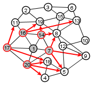
Given the above scenario, who will receive meme m from whom, and how many steps will it take for m to reach each person in the network? Answering these questions drives the distance algorithm.

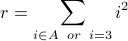
Example:

Node 9 is the source–the only node that starts with the meme

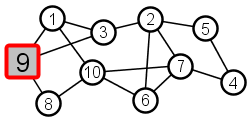
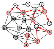
All nodes adjacent to 9 – nodes 1, 3, and 8 – receive the meme next. These nodes are distance 1 from source node 9.

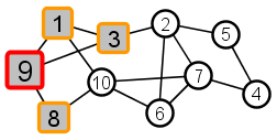
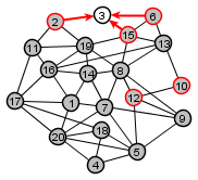
All nodes that are adjacent to 1, 3, or 8 and that have not already received the meme are next. These nodes – 2 and 10 – are distance 2 from source node 9.

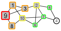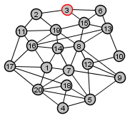
All nodes that are adjacent to 2 or 10 and that have not already received the meme are next. These nodes – 5, 6, and 7 – are distance 3 from source node 9.

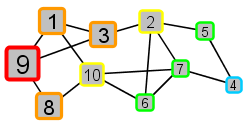All nodes that are adjacent to 5, 6, or 7 and that have not already received the meme are next. There is one such node – 4 – which is distance 4 from source node 9.

Computing distance, part two: Example

Below is another example that illustrates how to compute distance in a graph. It explicitly counts iterations (of the algorithm we will soon write) and it introduces some more formal bookkeeping: Set A_i = the set of nodes that are distance i from the source node.

For example:

is a set with one element: the source node.
is the set of all nodes adjacent to the source node.

Below we use A_i and a more complicated example to illustrate computing the distances from node 1 to every other node in the graph.

Beginning:

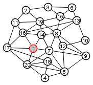Source node = 1

A_0 = Set of nodes that are distance 0 from source = {1}

Iteration 1:

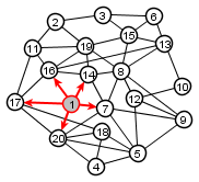Nodes not yet visited
all nodes except source
{2,3,4,5,…,20}
all white nodes

A_1 Set of nodes that are distance 1 from source
nodes adjacent to source
{7,14,16,17,20}
nodes with red arrows pointing at them

Iteration 2:

Updated set of nodes not yet visited {2,3,4,5,6,8,9,10,11,12,13,15,18,19} white nodes

A_2 = Set of nodes distance 2 from source unvisited nodes adjacent to any node in A_1 {4,5,8,9,11,13,18,19} nodes with red arrows pointing at them

Iteration 3:

Updated set of nodes not yet visited {2,3,6,10,12,15}
white nodes

A_3 = Set of nodes distance 3 from source
unvisited nodes adjacent to any node in A_2
{2,6,10,12,15}
nodes with red arrows pointing at them

Iteration 4:

Nodes not yet visited = {3}
A_4 = Set of nodes distance 4 from source
unvisited nodes adjacent to any node in A_3
{3}
nodes with red arrows pointing at them

Iteration 4:

Nodes not yet visited = { }
A_5 = Set of nodes distance 5 from source
unvisited nodes adjacent to any node in A_4
{ }

At the end of iteration 5, we see that there are no nodes distance 6 from the source node. Therefore, there are no nodes distance 7 from the source node, no nodes distance 8, etc.

Note that if a graph is not connected, then when the algorithm ends, only nodes in the same connected component as the source node will have been visited, and nodes in other components will not have been visited. Nodes that are still unvisited at the end of the algorithm are distance infinity from the source.