CSCI-1080 Intro To CS: World Wide Web
Saint Louis University, Department of Computer Science
Variables and Probability
Variables in mathematics
In mathematics, a variable represents a value.
Example: The following two equations use variables x and y. Furthermore, we can use algebra to determine the values of x and y.
x = 1
x + y = 3
Example: The following expression uses variable A, which represents a value that is precisely specified, fully known, and yet impossible for us to write down explicitly.
A = the set of all integers from 1 to 50 billion (inclusive)
Example: The following expression uses variable B, which represents a value that is precisely specified and yet impossible for us to know fully, much less write down explicitly.
B = the set of all people born in New Guinea during the year 5000 BCE
Example: The following expression uses variable C, which presents us with all the complications illustrated above and nags us once again with the question of how exactly to define “Web page”:
C = the set of all Web pages that –right now– have a hyperlink pointing to Amazon.com
Variables in algorithms
An algorithm may use a variable not only to represent a specific value but also to store information that changes according to the steps of the algorithm.
For example, the following algorithm uses variables  and
and  (which stand for “iteration” and “total”) to calculate
  when given any positive integer
  as input.
Algorithm to compute :
Input:
Integer n, with n  1
1
Output:
Variable t = the sum of all elements in the set {x: x is an integer and  }
}
Steps:
i = 0
t = 0
i = i + 1
t = t + i
if
 then we are done
go to step 3
Note: When considered purely as a mathematical expression, “ ” is clearly a false statement. No (finite) value of i will ever make “” a true mathematical expression. However, as a step in an algorithm, “” represents an action: “Add one to the current value stored in variable i.” Variable i stores information that changes according to the steps of the algorithm.
Random variables
In probability theory, a random variable represents an unknown value that may change each time it is observed.
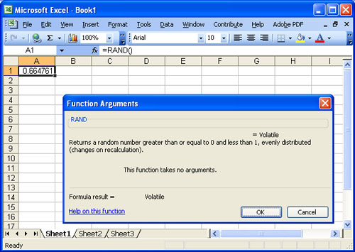
Example: Below is an Excel spreadsheet. The cell in row 1 column A contains the function RAND(). That cell is a random variable. Each time the spreadsheet is loaded, the value of that cell may change. According to the definition of RAND(), the value of the cell will be some decimal that is  and
and  .
.
Any time we observe the value of that cell, any value in that range is equally likely to be the result.
 |
Example: The result of rolling a 6-sided die is a random variable. Each time the die is rolled, the observed value may change. Any time we roll the die, any of the values 1, 2, 3, 4, 5, or 6 is equally likely to be the result.
Example: Suppose we choose one person from all the grown adults in the United States (each person being equally likely) and measure his or her height. The result is a random variable. Unlike the previous examples, some values are much more likely to occur than others. We would expect fairly often to observe a person's height  feet 8 inches. By comparison, we would expect very rarely to observe a person's height
  feet.
feet.
Discrete vs. continuous variables
Any variable may be discrete or continuous. In simplified terms the distinction is
A discrete variable has a finite set of possible values.
A continuous variable has an infinite set of possible values.
Examples:
Discrete: x is a positive integer no more than 10.
Discrete: x is a Web page.
Continuous: x is a decimal between 0 and 1. (There are infinitely many of these, e.g., 0.4901352…)
The set of all possible values for a variable is often called its domain. Our primary domains of interest are finite (e.g., people, Web pages). Hence we focus on discrete variables, using continuous variables when they allow us to simplify things.
(Readers wanting an unsimplified distinction of discrete and continuous should look up “countable” and “uncountable.”)
Probability distributions
Any random variable has a corresponding probability distribution that describes the likelihood of observing different values of that random variable.
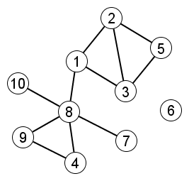
Example: The most famous probability distribution is the normal distribution (or “bell curve”), which is continuous:
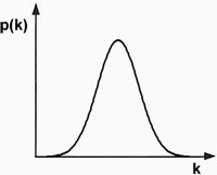 |
Normal distribution |
The height of grown adults follows a normal distribution. The x-axis (or “k”) in this figure above indicates possible height values; the y-axis (or “p(k)”) indicates the likelihood of observing a person of height k. The curve indicates that most people are average height; relatively few are short or tall; and no one is radically shorter or taller than average. (E.g., no one is 6 times taller than average.)
Example: Another common probability distribution is the uniform distribution, in which all possible values are equally likely. The uniform distribution below describes the process of rolling one die, which is discrete:
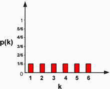 |
Uniform distribution. |
The set of all possible outcomes is {1,2,3,4,5,6}; each outcome has an equal probability of occurring, and the total probability of all possible outcomes must equal 1. Therefore:
p(k) = 1/6 if
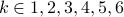
p(k) = 0 if
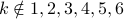
Example: The indegree of Web pages follows the power law distribution:
 |
Power law distribution. |
Most pages have low indegree, hence p(k) is large when k is small. A small but significant number of Web pages have extremely high indegree. These are the hubs of the Web graph. Sites such as Amazon and Wikipedia are notable hubs on the Web; each has indegree that is many thousands of times higher than average.
Note that the power law distribution is continuous, but Web pages and indegrees are discrete. Using the continuous power law distribution simplifies our analysis of the indegree of Web pages.
Degree distributions
Suppose we choose one node from an undirected graph (all nodes being equally likely) and measure the degree of that chosen node. The result is a random variable, and the probability distribution that describes that random variable is called the degree distribution of the graph.
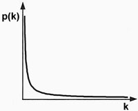
Example: Consider graph  drawn below. We calculate the degree distribution for this graph with the following 5 steps:
Measure the degree of each node in the graph–the “census.”
Find all the distinct degree values that result from the census.
For each distinct degree value, count how often it occurs in the census.
Divide the total number of occurrences of each degree value by the total number of nodes.
The resulting numbers represent the likelihood of each possible degree value: Draw the probability distribution.
 |
Let us compute the degree distribution of this graph |
Step 1:
| Vertex ID | Vertex Degree |
| 1 | 3 |
| 2 | 3 |
| 3 | 3 |
| 4 | 2 |
| 5 | 2 |
| 6 | 0 |
| 7 | 1 |
| 8 | 5 |
| 9 | 2 |
| 10 | 1 |
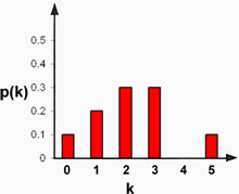
Step 2, 3 and 4:
| Degree value | How oftern occurs | Divided by |V| |
| 0 | 1 | 1/10 |
| 1 | 2 | 2/10 |
| 2 | 3 | 3/10 |
| 3 | 3 | 3/10 |
| 4 | 0 | 0/10 |
| 5 | 1 | 1/10 |
Step 5:
 |
Example: We use the same 5 steps to calculate the degree distribution of the graph drawn below. Notice that (1) the graph has a hub-and-spoke structure, and (2) the degree distribution of the graph is a rough discrete approximation of the power law distribution.
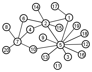 |
Step 1:
| Vertex ID | Vertex Degree |
| 1 | 3 |
| 2 | 6 |
| 3 | 1 |
| 4 | 2 |
| 5 | 10 |
| 6 | 2 |
| 7 | 7 |
| 8 | 1 |
| 9 | 1 |
| 10 | 2 |
| 11 | 0 |
| 12 | 1 |
| 13 | 1 |
| 14 | 1 |
| 15 | 1 |
| 16 | 1 |
| 17 | 1 |
| 18 | 1 |
| 19 | 1 |
| 20 | 1 |
Step 2, 3 and 4:
| Degree value | How oftern occurs | Divided by |V| |
| 0 | 1 | 1/20 |
| 1 | 12 | 12/20 |
| 2 | 3 | 3/20 |
| 3 | 1 | 1/20 |
| 4 | 0 | 0/20 |
| 5 | 1 | 1/20 |
| 6 | 1 | 1/20 |
| 7 | 0 | 0/20 |
| 8 | 0 | 0/20 |
| 9 | 0 | 0/20 |
| 10 | 1 | 1/20 |
Step 5:
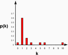 |
The contect of this site is licensed under a Creative Commons Attribution-ShareAlike 4.0 International License.