CSCI-1080 Intro To CS: World Wide Web

Saint Louis University, Department of Computer Science

Influence in Networks

Popularity, influence, and centrality

Our understanding of collective decision-making relies on the notions of popularity and influence. Popularity is the quality of being commonly liked; it is often used to measure the outcome of a collective decision (e.g., counting votes). Influence is the power to affect others; it is often used to shape the process of a collective decision (e.g., lobbying). These two distinct qualities are often combined – such as when popularity confers influence.

In the context of the Web, we mathematically model popularity and influence with indegree and PageRank™, respectively.

Indegree and PageRank™ are two ways of measuring network centrality. Despite its intuitive appeal, network centrality is hard to define. For example, which node is most central in the following graph?

There is no one right answer, because saying a node is “central” is ambiguous. A few ways to compute which node is most central include:

• Indegree Centrality: Just another way of saying indegree. Node 4 above has the highest indegree centrality: it is the only node with 3 incoming links.

• Outdegree Centrality: Just another way of saying outdegree. For a Web page, this indicates author activity. In the above graph, node 5 has the highest outdegree centrality: it is the only node with 3 outgoing links.

• PageRank™: An enhanced version of indegree centrality. In the above graph, node 2 has the highest PageRank.

In this chapter we will explain PageRank™, including the reasons why node 2 is most “influential” in the above graph. Our explanation combines basic concepts of set theory, graph theory, and algorithms – all drawn from previous chapters. Those who explore PageRank™ in more depth will find the literature full of references to matrix algebra and recursion, which are useful topics in more advanced courses of mathematics and computer science. For a head-first dive into these topics, see Eigenvector centrality, which is the mathematical foundation on which PageRank™ is built.

Introduction to PageRank

PageRank™ is Google's patented algorithm “to examine the entire link structure of the web and determine which pages are most important.” The details of the algorithm are secret, but the main ideas are well-known and much-copied.

The principles of PageRank™ are similar to those of a political election. In particular, a hyperlink from page x to page y counts as a “vote” cast by x for y. The rules of voting in this political election combine both democracy and oligarchy. The privilege of voting is open to all (democracy), but the weight of a vote depends on who cast it (oligarchy).

Famous features of PageRank™ include two ways votes are weighted:

• A vote from a high-ranked page is worth more than a vote from a low-ranked page.

• Each page can vote for any number of other pages; however, the weight of each of its individual votes decreases according to the total number of votes it has cast.

Most other parts of PageRank™ are closely guarded secrets. For example:

• Who has voted for whom? The contents of this ballot box are public, but who wants to count the votes? We rely on Google's database as a convenient substitute for verifiable vote-counting.

• Whose voting privileges have been revoked? As Web builders compete for PageRank™, some use techniques such as link-farming that Google considers to be cheating. Google works diligently and secretly to identify the cheaters and remove all their votes from the ballot box.

NetRank: a simplified version of PageRank

Here we present our own NetRank algorithm as a simplified version of PageRank™. NetRank and PageRank™ accept exactly the same input: a directed graph. They also provide the same kind of output – influence scores for all the nodes of the graph – although they compute slightly different values for these scores.

NetRank has two outstanding properties relative to PageRank™:

• NetRank captures the most important feature of PageRank™ that improves on indegree: Votes from high-ranked pages are worth more than votes from low-ranked pages.

• NetRank is much easier to compute than PageRank™ – mostly because NetRank ignores all the other ways that PageRank™ improves on indegree as a measure of influence.

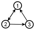
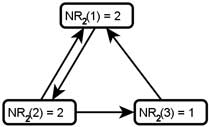
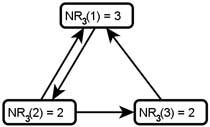
Example: We demonstrate the NetRank calculation using the following directed graph G=(V,E):

We write NR to denote NetRank. The calculation of NR proceeds iteratively. During iteration i, the calculation of improves upon the prior calculation of . We write to denote the NetRank value of node x during the iteration of the calculation.

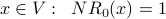
Iteration 0: To get the NetRank calculation started, we begin with for every node x. Below we redraw G and write each value inside the corresponding node.

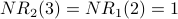
Iteration 1: For each node x, is the sum of the scores of all the nodes that vote for x:

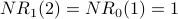
Below is G with each value drawn inside the corresponding node. Note that for each node x, equals the indegree of x. counts votes and gives every vote equal weight.

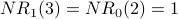
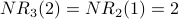
Iteration 2: For each node x, is the sum of the scores of all the nodes that vote for x:

counts votes, which are then weighted according to the rank of who cast each vote. is used as the basis for weighting. Here is G with each value drawn inside the corresponding node.

Iteration 3: For each node x, is the sum of the scores of all the nodes that vote for x:

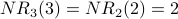
also counts weighted votes; however, the weighting of the votes is improved because is used instead of . Here is G with each value drawn inside the corresponding node.

Summary of Iterations 0-3: Each of the iterations above is a column in the following table:

Node x
1	1	2	2	3
2	1	1	2	2
3	1	1	1	2

Subsequent iterations: As we continue iterating, the pattern of computing by adding values remains the same. This pattern is determined by the original input to the algorithm: the nodes and edges of directed graph G. In our current example, the pattern can be drawn over the table of values. We also extend the table out to iteration 7:

The arrows show how values from one column move (or are added)
to determine the values in the next column.

Normalization and convergence

Here again is our example input to the NetRank algorithm:

The table below shows iterations 0-7 of the NetRank calculation for this graph:

Node x
1	1	2	2	3	4	5	7	9
2	1	1	2	2	3	4	5	7
3	1	1	1	2	2	3	4	5

The scores are different and bigger with each iteration. Evidently these numbers will change and grow for as long as the NetRank calculation continues to iterate. These observations lead us to two questions:

• In what sense are the influence scores improving with each iteration?

• How many iterations must be done before the algorithm can stop?

We answer these questions by introducing normalization and convergence.

Normalization is a calculation that makes it easier to compare one column of numbers to another column. Normalizing column of the above table involves two steps: (1) add the numbers in column , and (2) divide each of the numbers in column by that sum.

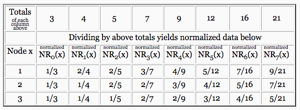The table above shows fractions to highlight the arithmetic of normalization. We write the exact same table a second time using decimals, in order to make it easier to compare one column of numbers to another (which is the point of normalization).

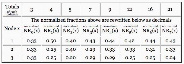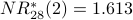
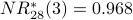
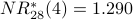
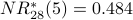
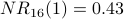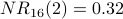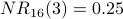Convergence is a property illustrated by the above table of decimals. With each iteration, the changes from one column to the next become smaller and smaller. If we were to expand the above table to show column , we would see that, after normalization, , , and . Furthermore, the normalized values would never change (to the nearest 0.01) after iteration 16.

This point – when further iterations of a calculation do not change the answer according to our desired level of precision (e.g., 0.01) – is the point of convergence.

By normalizing the results of the NetRank calculation, we find that after enough iterations the values will converge. How many iterations is enough depends on (1) our desired level of precision, and (2) the input graph. More precision and larger graphs will require more iterations for convergence to occur.

Conclusion: Having started with the following input graph:

We have used NetRank to calculate the relative influence of each node of the graph.

• The normalized NetRank score of node 1 is 0.43

• The normalized NetRank score of node 2 is 0.32

• The normalized NetRank score of node 3 is 0.25

The NetRank algorithm

Recall the NetRank calculation before we introduced normalization and convergence. For our 3-node example graph, we represented this calculation with the following table:

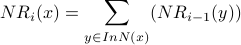
To write the NetRank algorithm (which computes the values in the above table), we need a mathematical way to say, “everyone who has voted for node x.” We define InNeighhorhood for this purpose.

Given a directed graph and a node x, the InNeighborhood of x is:

the set of all nodes with directed edges into x

We can now state the NetRank algorithm:

NetRank Algorithm:

Example: We will calculate iterations 0-5 of NetRank using the graph from the very beginning of this chapter:

The table below includes a column for the InNeighborhood of each node. As we see in step 3 of the algorithm above, this is exactly the information that determines the pattern of computing from . When constructing a NetRank table, writing this information explicitly helps organize the subsequent arithmetic.

Node x	InN(x)
1	{3,5}	1	2	3	5	10	18
2	{4,1}	1	2	5	8	15	26
3	{2,5}	1	2	3	7	11	22
4	{2,1,5}	1	3	5	10	16	32
5	{3}	1	1	2	3	7	11

The NetRank scores above have not been normalized. Skipping the process of normalization makes it impossible to detect convergence but easy to do a pre-specified number of iterations manually (without a calculator).

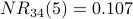
Node 4 is the most influential node according to . Using a spreadsheet, we can program the above calculation and include normalization. With a desired precision of 0.001, we observe convergence after 34 iterations. Node 4 is still the most influential node. The normalized NetRank values are:

• normalized

• normalized

• normalized

• normalized

• normalized

Dividing by outdegree: the NR* formula

One way to represent the NetRank calculation is with the NR formula:

For each node :

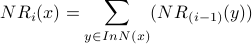
The NR formula is taken from step 3 of of the NetRank algorithm. In order to transform the NetRank calculation into PageRank™, we can keep the basic iterative structure of the NetRank algorithm, but we must make two changes to the NR formula:

1. Accounting for the following feature of PageRank™: For each page, the weight of each individual vote cast by that page decreases according to the total number of votes cast by that page.

2. Accounting for the “damping factor” that is built into PageRank™

The first change gives us the NR* formula:

For each node :

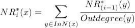
Besides renaming to , the only difference between the and formulas is that divides the weight of each vote by the outdegree of the node casting that vote. This models the desired effect: the weight of each individual vote cast by a page decreases according to the total number of votes cast by that page. Intuitively, if a website links to your site but also links to a lot of other sites, then its outdegree is high, so the fact that it links to your site is not that relevant. If instead the site links to very few sites and yours is one of them, (i.e., small outdegree) then all its outgoing links are more “important”.

Example: We will calculate iterations 0-5 of with the same graph we just used to demonstrate :

The table below includes a column for the outdegree of each node. Because each calculation adds fractions with different denominators (based on outdegree values), the arithmetic is too messy to do manually. We have used a spreadsheet to calculate the - values below.

Node x	Outdegree(x)	InN(x)
1	2	{3,5}	1	0.833	0.597	0.597	0.660	0.652
2	2	{4,1}	1	1.500	1.750	1.625	1.604	1.594
3	2	{2,5}	1	0.833	0.917	1.014	0.965	0.971
4	1	{2,1,5}	1	1.333	1.333	1.306	1.264	1.301
5	3	{3}	1	0.500	0.417	0.458	0.507	0.483

The scores above have not been normalized; however it appears that scores will converge even without normalization. This convergence occurs because dividing by outdegree has an effect similar to that of normalization. In particular, dividing by outdegree limits how much the values can grow – unlike the endless growth of NR values that we have observed.

Note: Using instead of gives us a different definition of the most influential node in our graph. Node 2 is the most influential node according to . Using a spreadsheet, we can program the above calculation with a desired precision of 0.001 and observe convergence after 28 iterations. Node 2 is still the most influential node. The NR* values are

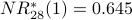
Previously we have seen that node 4 is most influential according to ; it is second-most influential according to .

Consider: Why does node 4 drop from most influential to second-most influential after we account for outdegree in the weighting of votes?

The PageRank formula

We create PageRank™ (PR for short) by adding a “damping factor” to the formula. The damping factor d is a fixed decimal value, (e.g., ).

The PR formula:

For each node :

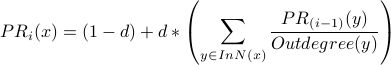
Besides renaming to , the only difference between the and formulas is the use of the damping factor d. The meaning of the damping factor is subtle, so we first note what happens if we choose the most extreme possible values of d:

• If then and are exactly the same formula.

• If then and the rest of the formula is irrelevant.

Example: We will calculate iterations 0-5 of PR, using and the same graph as before:

Node x	Outdegree(x)	InN(x)
1	2	{3,5}	1	0.858	0.678	0.686	0.719	0.715
2	2	{4,1}	1	1.425	1.606	1.529	1.518	1.513
3	2	{2,5}	1	0.858	0.919	0.978	0.953	0.955
4	1	{2,1,5}	1	1.283	1.283	1.266	1.245	1.261
5	3	{3}	1	0.575	0.515	0.540	0.566	0.555

The PR scores are very similar to the NR* scores. Using a spreadsheet, we can program the above calculation with a desired precision of 0.001 and observe convergence after 13 iterations. Node 2 is still the most influential node. The PR values are

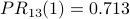
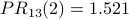
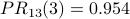
The damping factor: PageRank as probability

In order to understand what the damping factor means, it helps to reframe our PageRank™ metaphor from a political election to a Web-surfing monkey.

PageRank™ provides a kind of probability distribution for the following random variable: If a monkey were to sit down at a browser and start clicking and typing, what Web page would be left on the screen when the zookeeper finally takes the monkey away from the computer? PageRank™ tells us the likelihood that any specific page will be the monkey's final destination.

Now suppose we also know how often the monkey likes to click on a random link vs. how often the monkey likes to type a random URL into the browser. In this scenario, the damping factor d expresses the monkey's preference for clicking instead of typing. So…

• If then the resulting PageRank™ function assumes that the monkey starts at a random page and then always clicks and never types in a new URL.

• If then the resulting PageRank™ function assumes that the monkey never clicks; it always types in another random URL.

Admittedly the model corresponds to an unrealistic and-or pathological version of Web surfing – equivalent to the famous team of monkeys still typing up King Lear. Hence our best intelligence says that Google uses , which is closer to 1 than 0.