CSCI-1080 Intro To CS: World Wide Web

Saint Louis University, Department of Computer Science

Network Dynamics

Limitations of traditional graph theory

Conceived in 1735 by the fertile Leonhard Euler, graph theory developed over the next 200 years to include topics such as:

• Shortest paths: Given a graph and a pair of nodes x,y: How can we find a shortest path from x to y?

• Maximum cliques: A clique is a subset of nodes that are all adjacent to each other. Given a graph : How can we find large cliques in G? How can we find the largest clique in G? (Please refer to the network structure page for a more thorough definition of clique.)

• Graph coloring: Given a graph and the ability to assign a “color” to each of its nodes: How can we use the fewest possible number of distinct colors so that (1) every node has a color assigned to it, and (2) no two adjacent nodes are assigned the same color?

In studying these and other questions, graph theorists usually made two important assumptions: (1) The graph is known, and (2) the graph does not change.

When we use graph theory to study the Web, we must acknowledge that these two assumptions are not realistic. For example:

• The Web graph is only partially known. Estimating the cardinality of the set of all Web pages is enough to stretch our powers of creative arithmetic; what if we actually had to name all 30-70 billion of them? Our knowledge of the set of all hyperlinks is rougher still.

• The Web graph is constantly changing. Even if all Web builders were to cease and desist immediately, the Web pages they have already created include many that automatically change their outgoing links each time a Web user visits. For example, Google, Facebook, Amazon, etc. all present different links to different users at different times.

Introduction to network dynamics

In the 1940s and 50s, graph theory expanded in important ways to strengthen our understanding of network dynamics. Two notable milestones were:

1. Studying dynamic flows: commodities that move over predetermined graphs. During World War II, a great deal of attention was paid to questions such as: “How do we get supplies to our soldiers despite our enemies’ attempts to stop us?” Here nodes represent sources, destinations, and transfer stations for commodities such as food, fuel, ammunition, and medicine. Edges represent roads and other means of transport between pairs of nodes.

2. Studying dynamic graphs: sets of nodes and edges that change over time. Just after World War II, for reasons much more theoretical than supplying troops, mathematicians formalized the study of graphs whose very nodes and edges change over time. For example, if a graph started with 1,000 nodes and no edges, and then edges were added randomly one at a time to join those 1,000 nodes, what could we say about the evolving properties of that dynamic graph? Both types of network dynamics are important to understanding the Web. For example:

   1. Information flows through the Web via the Internet. Typically, Web hosts provide information, Web browsers request and receive information, and Internet routers are transfer stations. Internet connections such as cables and wi-fi correspond to edges.

   2. The Web is an ever-changing collection of pages and links. So many Web pages and hyperlinks are being added and edited at this very moment that any attempt to catalog them would be outdated before it could be completed. Pages are also removed from the Web (either temporarily by service disruptions or permanently by decommissioning), resulting in “dead links” and other complications that frustrate our hope to know the Web.

Our discussion here will focus on the second type of network dynamics: What are the evolving properties of the Web as millions of people continually edit its pages and hyperlinks? This is a core question in the realm of Web Science.

The first type of network dynamics–how information flows through the Web–is no less important than our chosen focus. We defer its discussion for two reasons: (1) The question of how information can best move right now from a Web host to a Web browser, known as packet-routing, has been well-studied in the realm of traditional Computer Science, where we can use it as a “black box”; and (2) The question of how information spreads over time through populations of Web users (e.g., information diffusion) is more advanced than the material presented here.

Also, in focusing on the ever-changing Web, we will ignore dynamic pages such as Google, Facebook and Amazon, that present different links each time a user visits. We will focus on static pages that millions of regular Web builders make every day with HTML and CSS. What do we learn when we view each of those pages not as an isolated artifact but as a crossroads in a network of millions of Web users and builders?

Random Graphs

Chapter 2 of Six Degrees starts with an excellent introduction to random graphs. Have that handy before you continue.

Random graphs (and their dynamics) are based on the following assumptions:

• The graph we start with has many nodes but no edges.

• Edges are added randomly one at a time to the graph. (I.e., any pair of non-adjacent nodes is equally likely to be the next edge added to the existing graph.)

• Eventually, we end with a clique: every pair of nodes is adjacent.

Given the above framework, how does a graph evolve between the starting and ending points? That is a core question of random graph dynamics.

One of the most famous results in the dynamics of random graph describes the size of the largest connected component, also called the giant component. Read in Six Degrees the explanation of Figure 2.2 on p. 45. A similar figure labeled with our own terminology is below:

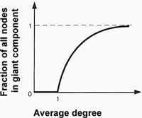After you absorb Six Degrees, then consider what this means:

• By eyeballing the above figure, we can estimate that a random graph with average degree of 2 has a giant component with 75% of all nodes.

• Whether |V| is big or small doesn't matter at all: To connect a set of nodes into a giant component, just randomly add |V| edges and you have guaranteed that the average degree is at least 2, thus creating a giant component with 75% of all nodes.

Example: Suppose all links are deleted from the Web. Only the 30-70 billion link-less pages remain. If each author of each Web page added just one random link to each of his pages, then the resulting giant component would connect 75% of all Web pages into a giant component connected by undirected paths (which allow both forward and backward traversing of hyperlinks).

Random graph algorithm

An algorithm is a set of instructions that explain how to compute something. It is like a recipe, only for making data instead of food.

An algorithm has three parts:

1. Input (like the ingredients of a recipe)

2. Output (like the title of a recipe: “chile con carne, serves 12”)

3. The steps of the algorithm (like the steps of the recipe)

The following algorithm describes the creation of a random graph.

Random Graph Algorithm:

Note: The main point of most algorithms is generating output, just as the main reason for most recipes is serving food. For example, a sorting algorithm is useful as a way to alphabetize names, and Google's PageRank algorithm is useful as a way to list the most popular and influential Web pages first.

Our random graph algorithm, however, does not generate interesting output. It creates a clique using a more complicated sequence of steps than is necessary to create a clique. The point of the algorithm is the journey it describes, not the destination where it eventually arrives.

Clusters and homophily

Informally speaking, a cluster is a group of nodes in a graph that are more connected to each other than they are to the rest of the graph. For example, the red and yellow regions below are clusters:

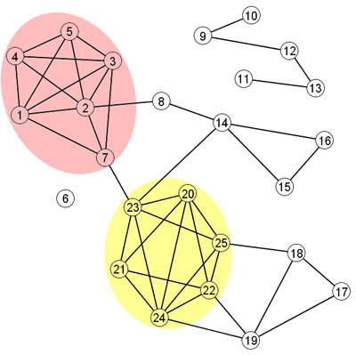Clusters provide a good big-picture view of the Web, much like a table of contents provides a big-picture view of a book. Unlike a book and its table of contents, however, a cluster involves many authors (Web builders) acting independently. Also, a Web builder may be unaware of the clusters he is forming.

The sociological force behind Web clusters is homophily, or “birds of a feather” (which “flock together”). Here is one important way that homophily impacts the Web:

1. When a Web builder links from his site to another site, he usually does so because he perceives something important shared by his site and the other site.

2. Therefore hyperlinks represent more than channels of navigation; they also represent shared likes and dislikes.

3. The navigational meaning of a hyperlink is clear and explicit, but the shared likes and dislikes represented by a hyperlink are often unstated and implicit.

4. Therefore clusters of mutually interlinked Web pages represent self-organized groups with specific shared likes and dislikes, which are usually unstated and implicit.

Motivated by the above, cluster-based search engines find interlinked groups of Web pages and then deduce the specific “meaning” of each cluster by analyzing the content of the interlinked pages. An example of cluster-based search engines is iBoogie.

Triadic closure

Triadic closure is a simple and effective mathematical model of homophily in a network. The basic idea is illustrated below:

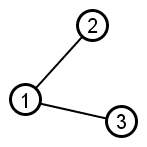Nodes 2 and 3 share a mutual neighbor but are not adjacent.

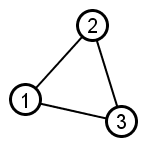Adding edge {2,3} is then an example of triadic closure.

Triadic closure usually occurs in the context of a larger graph. For example, in the graph below–considering only the solid black lines as edges–there are many possible opportunities for triadic closure. Just a few of those possible opportunities are illustrated with dotted red lines.

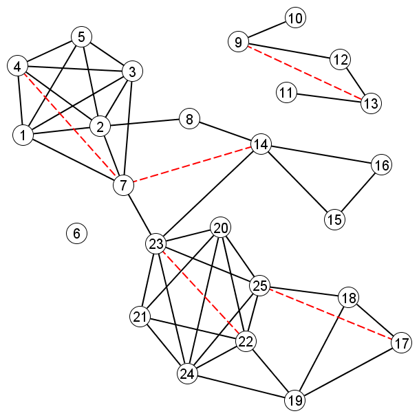Triadic closure algorithm

Chapter 2 of Six Degrees pp 56-61 has a good introduction to homophily and triadic closure. Read that before you continue. The following algorithm describes the process of repeated triadic closure:

The output of the triadic closure algorithm has some notable properties. We can deduce these properties from the following observations:

Consider the closing of a single triad: Nodes x and y are non-adjacent and share a common neighbor; then x and y are joined by edge {x,y}.

1. Adding edge {x,y} does not change the number of connected components in G. Nodes x and y were already connected before we joined them with {x,y}.

2. Adding edge {x,y} increases the density of the connected component that contains nodes x and y.

Repeating the above observations over the course of every iteration of the triadic closure algorithm, we see that the output graph G’=(V,E’) computed by the algorithm has these two properties

1. Output graph G’ has exactly the same number of connected components as input graph G. Furthermore, the nodes that induce each connected component are the same in G’ and G.

2. Each connected component of G’ has the maximum possible density: it is a clique.

Example: Suppose the triadic closure algorithm starts with graph G=(V,E) drawn below:

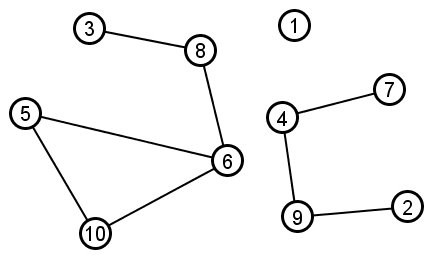Upon completion, the algorithm will have added all the orange edges drawn below:

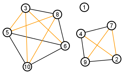The output graph has the same number of connected components as the input graph (with the same nodes in those components). And each connected component in the output graph is a clique.

An algorithm that identifies and closes triads is an example of random-bias. A network resulting from that algorithm is an example of randomly-biased network (graph). Intuitively, a random-biased network is a network that obeys to some property but it is otherwise random. In the triadic closure example, the bias is towards closing a triad (adding an edge) if two nodes have already a common neighbor; the two nodes with the common neighbor are selected however at random.

Hubs and cumulative advantage

A hub is a node in a graph with much higher degree than average. For example, nodes 1 and 2 are both hubs in the figure below:

Centrality is the mathematical term most commonly used to describe hubs. Degree and indegree are two common simple measures of centrality.

Google made centrality-based Web search famous, and centrality-based search engines now dominate the Web. If cluster-based search engines reveal something like a Web “table of contents,” then centrality-based search engines provide quick shortcuts to “the good parts”–the most popular pages and pictures.

The sociological force behind Web hubs is cumulative advantage, or “rich get richer.” Here is one important way that cumulative advantage impacts the Web:

1. When a Web builder is looking for online resources, he probably uses a centrality-based search engine like Google, and he is more likely to look at higher-ranked pages.

2. Pages atop centrality-based rankings are there because they are already popular (essentially because they have high indegree.)

3. Therefore Web builders are more likely to link to (and increase the indegree of) pages that are already popular. It is possible that Web builders will never even see the “good” pages that are not popular.

4. Therefore Google and its ilk, to some extent, drive a feedback loop that amplifies the popularity of whatever is already popular. In other words, the rank of a Web page next week has less to do with its content and more to do with its rank this week. The main change to be expected in next week's rankings is that disparities between high rankings and low rankings will increase. The rich get richer.

Preferential attachment algorithm

Chapter 4 of Six Degrees pp 108-109 has a good introduction to cumulative advantage (known also as “rich get richer” and the “Matthew effect” among other names) and its effect on network dynamics. Read that before you continue.

Preferential attachment is the mathematical model used to represent the force of cumulative advantage in network dynamics. The algorithm below describes the process of repeated preferential attachment. This is equivalent to the algorithm informally described on pp 108-109 of Six Degrees:

Preferential Attachment Algorithm:

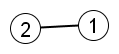
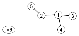
Example: Suppose the preferential attachment algorithm starts with , , and n=20. Therefore k=2 and the input graph can be drawn as:

The sequence below illustrates the first few iterations of the algorithm.

Iteration 1

Create node 3 and join it to a pre-existing node. Node 1 and node 2 are equally likely.

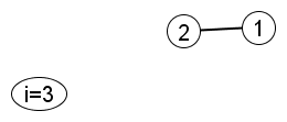Suppose the algorithm joins node 3 to node 1. Then…

Iteration 2

Create node 4 and join it to a pre-existing node. Node 1 is twice as likely as node 2 or node 3.

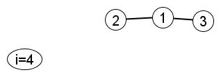Suppose the algorithm joins node 4 to node 1. Then…

Iteration 3

Create node 5 and join it to a pre-existing node. Node 1 is 3 times as likely as node 2, 3 or 4.

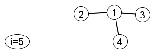Suppose the algorithm joins node 5 to node 2 (i.e., a lucky break for node 2). Then…

Iteration 4

Create node 6 and join it to a pre-existing node.

Iterations continue…

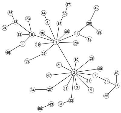
In the very last iteration, node 20 is joined to node 2

Output graph:

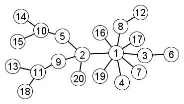Notice in the above example that nodes 1 and 2 start out as equals. However, the random choice of node 1 in the first iteration gives node 1 a nudge up in popularity that feeds on itself. In the end, node 1 is the single dominant hub and node 2 is a second-tier mini-hub.

A seemingly insignificant event in iteration 1 has caused a very substantial effect because of cumulative advantage.